

The following publication has been lightly reedited for spelling, grammar, and style to provide better searchability and an improved reading experience. No substantive changes impacting the data, analysis, or conclusions have been made. A PDF of the originally published version is available here.
As specified in the 1977 amendment to the Federal Reserve Act of 1913, the Federal Reserve System and the Federal Open Market Committee (FOMC) should conduct monetary policy to promote the goals of maximum employment and output and to promote stable prices. Of these goals many people believe that the primary focus should be on achieving price stability. A stable price level means that prices of goods are undistorted by inflation and so can serve as clearer signals to promote the efficient allocation of resources and the maximum possible sustainable level of employment. It is also believed that a stable price level encourages saving and capital accumulation because it prevents asset values from being eroded by unanticipated inflation. This should contribute to the first two goals.
For these reasons the conduct of monetary policy is heavily influenced by factors thought to influence the rate of change of prices, i.e., inflation. Since the main experience in living memory is of generally rising prices and episodes of high inflation that have been associated with bad macroeconomic outcomes, most attention currently is focused on keeping inflation from accelerating. Given the long lags over which policy actions can take effect, it is often necessary for the FOMC to take action before inflation starts to rise. The only way to do this with some confidence is to have effective ways of predicting future inflation. Hence forecasting inflation is a crucial ingredient in the formulation of monetary policy.
In this Fed Letter, I discuss a new approach to inflation forecasting rooted in a traditional statistical framework.1 This approach is based on recent research by James Stock of Harvard University and Mark Watson of Princeton University.2 The methods these researchers have proposed involve harnessing the information contained in the large number of variables that economists look at in real time when trying to assess the state of the economy.
To appreciate the potential benefits of the new methods we need to understand the standard approach to statistical inflation forecasting. This involves estimating how inflation in the past has been related to other variables, called inflation indicators, which have had predictive power for inflation in the past. Faced with the large number of data series available in real time, forecasters tend to focus on a small number of inflation indicators.
The first issue when constructing a forecasting model, then, is deciding what makes a good inflation indicator. To help illustrate this, figure 1 plots the 12-month rate of change of the core Consumer Price Index (CPI) quarterly from 1963 to 1999. The shaded regions marked with Roman numerals cover episodes during which this measure of inflation has risen for extended periods of time, defined here to be at least one year of roughly continual growth. Episodes I, II, and III are the great inflations associated with the Vietnam War and the two oil shocks. Notice that these episodes are much more dramatic than the last four in the figure. In fact, you almost need a magnifying glass to see the two short episodes of rising inflation in the 1990s.
1. Core inflation with episodes of rising inflation
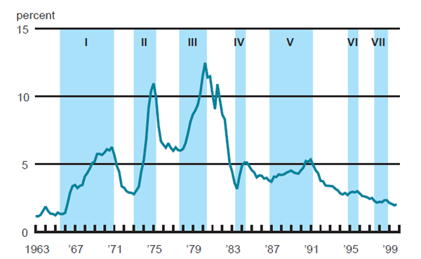
Source: U.S. Department of Labor, Bureau of Labor Statistics, 1963–99, “Consumer Price Index for all urban consumers, less food and energy component,” available on the Internet at http://stats.bls.gov/top20.html#CPI.
What would make a good indicator of core CPI inflation? When formulating monetary policy, we need to know whether inflation is likely to pick up in the future. So, we need variables that display a consistent pattern in the periods leading up to each of these shaded regions. The more consistent the pattern, the better the indicator. When this is the case, statistical models will have consistent, systematic information to predict inflation.
The classic and most watched indicator of inflation is the civilian unemployment rate. In figure 2 the civilian unemployment rate is plotted from 1963 to 1999. The shaded regions are the same as in figure 1. One key thing to notice from this figure is that in the periods leading up to most of the episodes, the unemployment rate has tended to fall from relatively high levels to relatively low levels at least a year before the episode. This is most apparent for the first three episodes, which involved the most pronounced accelerations in inflation (see figure 1). No indicator is perfect. For example, it is hard to say that the fourth episode, with the rising unemployment from a high level preceding it, is similar to the first three in which unemployment fell from a high level. Nevertheless, the general pattern of falling unemployment before rising inflation is why the unemployment rate, at least until recently, was one of the best inflation indicator variables among the thousands available.
Many observers have mentioned the difficulties standard inflation models have had in recent times, and we can see why in figure 2. The dramatic fall in unemployment over the last eight years is similar to that seen in previous periods. In the past, these dramatic declines were followed by equally dramatic outbursts of inflation. Yet the two episodes from the 1990s, were minuscule (see figure 1). Another gauge of the unreliability of unemployment as an indicator is that its trend rate, sometimes called the natural rate, seems to change over time— it is relatively low in the 1960s, high in the 1970s and 1980s, and low again in the 1990s.
2. Unemployment with episodes of rising inflation
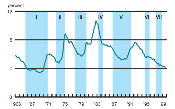
Source: U.S. Department of Labor, Bureau of Labor Statistics, 1963–99, “Civilian unemployment rate,” Washington.
The experience with unemployment is common to the many widely used indicators, including capacity utilization, interest rate spreads, and producer prices. Generally, the widely used indicators do well in some periods and less well in others, and often a relationship that is pronounced at one time disappears in later episodes. Ultimately, this is because inflation is a very complicated phenomenon, determined by many factors. Any single data series may appear useful for a while only because its behavior is by chance aligned with inflation’s basic determinants. As the economy evolves, this fortuitous relationship may break even if the basic determinants of inflation have not changed.
To accommodate this fact, one might imagine that all we need do is include all the best inflation indicators in our statistical model. But the conventional way of doing this is problematic. There are many good inflation indicators, and statistical models behave erratically when they include many variables. In fact, including many variables can lead to disaster, generating forecasts that look like nonsense. So, we have many useful indicators, each containing some information about inflation, but we cannot use them all and individually they are unreliable.
The new research by Stock and Watson suggests a way out of this conundrum. The idea behind their approach is that there is some component common to the inflation indicators, and it is this common component, or index, that is useful for predicting inflation. If we can identify this index, then we have a way to incorporate the information in a large number of good inflation indicators, without overburdening our forecasting models. Specifically, identify the common component of many indicators and then put this single variable in the forecasting model.
Stock and Watson provide a way to estimate the index that can be applied to any number or type of indicators. For example, it can be used to identify the common component in financial variables, in price series, in consumption series, in labor markets, in the manufacturing sector, even all these variables put together. The basic idea involves finding a weighted average of the series under consideration that explains as much of the combined variation in these series as possible.3
Recent research shows that, from the perspective of inflation forecasting, an index derived from one particular set of indicators appears to have a lot of promise. This is a set of data series each of which measures some aspect of overall macroeconomic activity. The Chicago Fed has begun compiling a version of this index on a real-time basis using over 70 series, including aggregate and sectoral data on labor market conditions (24 series), industrial production (20 series), inventories, new orders and housing (16 series), personal income and consumption expenditures (7 series), and manufacturing and trade sales (9 series). In the spirit of the unemployment rate, which by the way is included in the index, one can think of the derived series as a generalized measure of the temperature of the economy. Stock and Watson call it the “Activity Index.”
To gauge the sense in which the Activity Index actually measures overall activity in the economy, figure 3 shows the Activity Index along with shaded regions corresponding to the five recessions (as defined by the National Bureau of Economic Research) that have occurred since 1962. Notice that the five lowest values of the index roughly indicate the troughs of the five recessions (the last period of each shaded region in the figure).
3. Activity Index with NBER-dated recessions
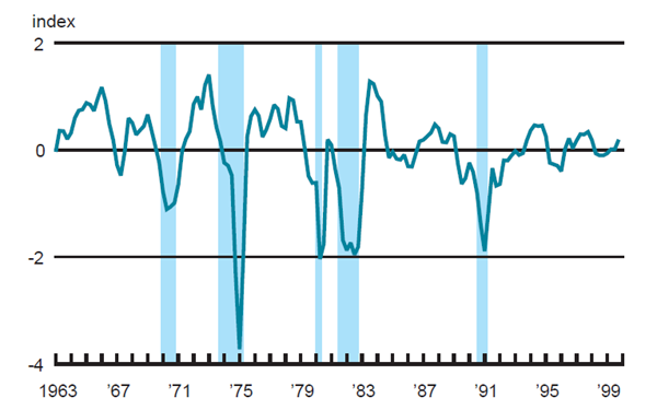
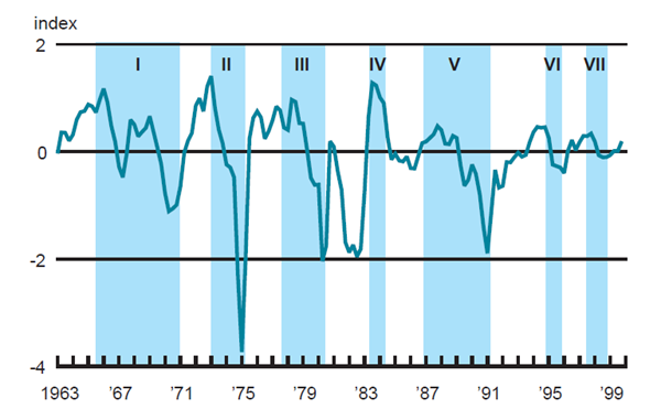
Figure 4 shows the Activity Index along with the shaded rising inflation episodes as in figures 1 and 2. Notice how the index rises before each of the episodes. This is the sort of pattern we look for in a good inflation indicator. As with unemployment, there is early indication of inflation in episodes I, II, and II. Episode IV seems to have been less of a surprise for the Activity Index than it was for unemployment (see figure 2), and the last three episodes are also well predicted in that the index rises before each of these inflationary outbursts.
One indication of the potential quality of the index as an inflation indicator is that its increases leading into the last three episodes, V, VI, and VII, seem smaller than for the first three. Unlike unemployment, then, this appears to be consistent with the smaller magnitude of the inflationary outbursts in these later periods (see figure 1). This may be a sign that the Activity Index is coping well with the “new economy” everyone is talking about.
Figure 4 is intended to provide an indication of the potential for the Activity Index to forecast inflation. Another way to build confidence is to perform out-of-sample forecast tests. Stock and Watson perform such tests with a version of the Activity Index. They compare the Activity Index to a large number of alternative indicators within the context of a single equation forecasting framework, in which inflation is related to lagged inflation and lags of various indicator variables. Included in the set of models they examine are the commonly used nonaccelerating inflation rate of unemployment (NAIRU) and potential output models.4 They also examine many indexes constructed using the same techniques as the Activity Index. A key finding from their research is that across different time periods and measures of inflation, the Activity Index, or something very close to it, is found to beat any other single indicator or combination of forecasts coming from using different indicators. Research at the Chicago Fed generally supports these findings.
4. Activity Index with episodes of rising inflation
The Stock and Watson forecasting strategy has other benefits beyond pure forecasting performance. They have demonstrated that their common component procedure has many desirable theoretical properties, including an ability to accommodate structural change. From a practical perspective, it does not place too much weight on any one series, which seems sensible. It is also particularly well suited for real-time analysis because it can accommodate data that are released at different times and frequencies.
Conclusion
In sum, research, theory, and plots like figure 4 suggest that something like the Activity Index may prove to be a valuable tool for forecasting inflation. However, many issues still need to be resolved. For example, while the calculation of the index is straightforward, finding the most appropriate statistical framework to incorporate the information in the index is more problematic. Another issue is that the method for selecting the variables in the Activity Index was essentially ad hoc. A systematic procedure for identifying the best series to include in the index may yield even better results. Addressing these and related issues is the focus of ongoing research at the Chicago Fed.
Tracking Midwest manufacturing activity
Manufacturing output indexes (1992=100)
| December | Month ago | Year ago | |
|---|---|---|---|
| CFMMI | 137.5 | 136.8 | 131.3 |
| IP | 145.5 | 145.2 | 138.4 |
Motor vehicle production (millions, seasonally adj. annual rate)
| January | Month ago | Year ago | |
|---|---|---|---|
| Cars | 5.7 | 5.6 | 5.6 |
| Light trucks | 7.1 | 6.9 | 6.8 |
Purchasing managers' surveys: net % reporting production growth
| January | Month ago | Year ago | |
|---|---|---|---|
| MW | 51.4 | 58.1 | 51.6 |
| U.S. | 55.9 | 59.0 | 53.7 |
Motor vehicle production (millions, seasonally adj. annual rate)
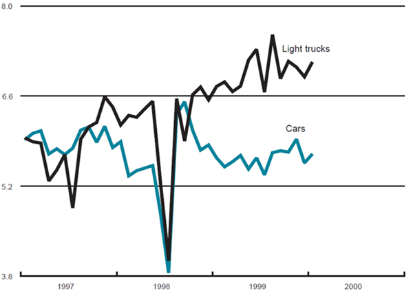
Light truck production increased from 6.9 million units in December to 7.1 million units in January, and car production also increased from 5.6 million to 5.7 million units from December to January.
The CFMMI rose 0.5% from November to December, reaching a seasonally adjusted level of 137.5 (1992=100). In comparison, the Federal Reserve Board’s IP increased 0.2% in December, after rising 0.6% in November. The Midwest purchasing managers’ composite index (a weighted average of the Chicago, Detroit, and Milwaukee surveys) for production decreased to 51.4% in January from 58.1% in December. The purchasing managers’ index decreased in Chicago and Detroit but increased slightly in Milwaukee. The national purchasing managers’ survey for production decreased from 59% to 55.9% from December to January.
Notes
1 This article is a revision of a speech to the joint meeting of the Boards of Directors of the Federal Reserve Banks of Chicago and Cleveland on October 28, 1999.
2 The key references are “Diffusion indexes” and “Forecasting inflation” which are both 1999 Princeton University working papers by James Stock and Mark Watson.
3 Technically, the index can be derived from the first principal component of the moment matrix of the series. Stock and Watson consider the possibility that more than one underlying component drives inflation. These other components are also derived using principal components analysis.
4 NAIRU models relate inflation to the difference between the unemployment rate and its trend. Potential output models are similar in spirit, but inflationary pressure is expressed in terms of the difference between output and some level of output called potential.


