

We describe a new set of indexes—the Brave-Butters-Kelley Indexes (BBKI)—constructed from a large panel of monthly macroeconomic time series and quarterly real gross domestic product (GDP) growth. Through August, these indexes suggest that real GDP growth was somewhat below its long-run trend to start the third quarter and that its business cycle component had declined noticeably in recent months despite some indications of improvement in its leading indicators.
Earlier this year, a new “big data” activity index was introduced in an Economic Perspectives article.1 This index was constructed from 500 monthly measures of growth in U.S. economic activity and quarterly U.S. real GDP growth. To recap that work, the authors developed what is referred to as a mixed-frequency collapsed dynamic factor model2 that allowed for the estimation of the unobserved monthly evolution of quarterly U.S. real GDP growth based on the variation in a panel of 500 monthly time series. Included in this panel were the coincident, leading, and lagging monthly real activity indicators commonly used to assess the state of the business cycle for the United States. Using this model, the authors then decomposed monthly real GDP growth into three separate components: trend, cycle, and irregular components. The big data activity index represented the cycle component of this decomposition and was shown to have several highly desirable properties, including being 99% accurate in aligning with historical U.S. recessions and expansions as defined by the National Bureau of Economic Research (NBER) since 1960.3
In this Chicago Fed Letter, we provide updated estimates based on their model and discuss the implications for the current state of the U.S. economy. On November 4, 2019, we will begin releasing these new measures of monthly real GDP growth and its components, constituting what we are now calling the Brave-Butters-Kelley Indexes, on a monthly basis. Through August, BBK Monthly GDP Growth suggests that real GDP growth was slightly below its long-run trend to start the third quarter, with its cycle component declining noticeably in the past few months. However, recent improvements in the cycle’s subcomponent attributable to its leading indicators also suggest that some of the weakness in growth may be expected to abate over the next few quarters.
Monthly real GDP growth
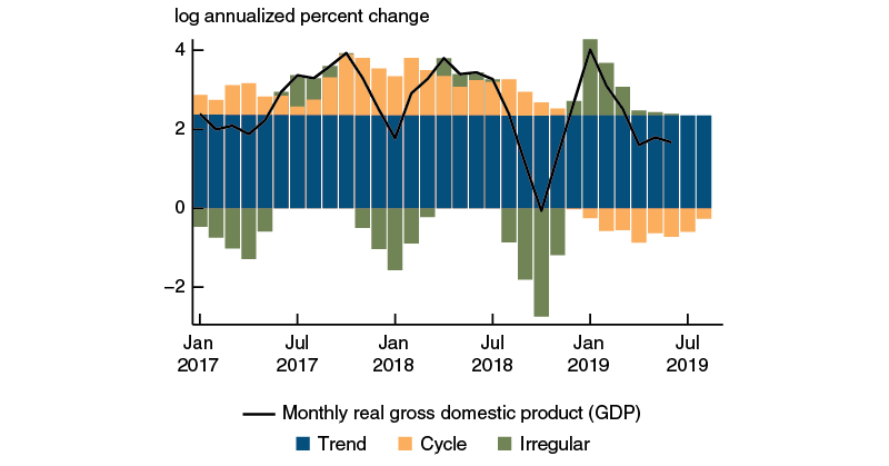
Figure 1 shows an updated estimate of BBK Monthly GDP Growth, which is indexed to the quarterly estimates of real GDP growth from the U.S. Bureau of Economic Analysis. It is decomposed in the figure into its trend, cycle, and irregular components since 2017. The trend component captures slow-moving changes in average real GDP growth over time and, as such, is shown in figure 1 on an annualized (log) percent change basis to be about 2.3% in August 2019.4 In contrast, the irregular component captures short-run deviations around this trend that are highly mean-reverting, or short-lived.5 Meanwhile, the cycle component captures more persistent medium-run deviations characteristic of the business cycle.6
1. Decomposition of Brave-Butters-Kelley Monthly GDP Growth, 2017−19
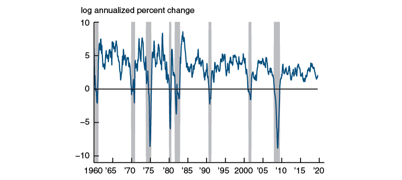
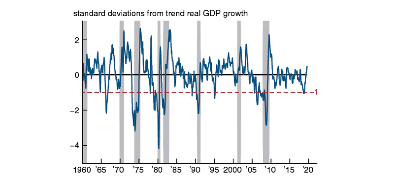
To highlight the persistent components alone (i.e., after the irregular component is removed), we plot in figure 2 the sum of the estimated trend and cycle components for BBK Monthly GDP Growth over a longer time period. Through August 2019, these two components were consistent with an annualized (log) real GDP growth rate of 2.1%, representing a fairly significant decline from the 3.8% rate observed in early 2018, but still well above the negative growth rates historically associated with U.S. recessions as seen in the figure. This point is made even clearer by figure 3, which instead focuses on only the cycle component. Here, we refer to it as the BBK Coincident Index, reexpressing it in standard deviation units from trend real GDP growth and noting its rule-of-thumb threshold value for identifying business cycle turning points as a dashed red line.7 At –0.3 standard deviations, the current value of this index is still well above the –1 value that has historically been associated with an elevated likelihood of a recession.
2. Brave-Butters-Kelley Monthly GDP Growth: Trend and cycle components
Source: Authors’ calculations based on data from Haver Analytics.
3. Brave-Butters-Kelley Coincident Index

Source: Authors’ calculations based on data from Haver Analytics.
The subcomponent of the cycle attributable to its leading indicators is shown separately in figure 4, where it is also expressed in standard deviation units from trend real GDP growth and is referred to as the BBK Leading Index. In addition, its own rule-of-thumb threshold value at a lead of eight months relative to business cycle turning points is shown in the figure as a dashed red line. It is readily apparent from figure 4 that using this leading index to predict recessions is likely to produce many more false positive and false negative signals than the contemporaneous signal provided by the BBK Coincident Index (see figure 3). The BBK Leading Index’s current value remains well above the –1 standard deviation threshold that has historically tended to signal an elevated likelihood of a recession eight months hence. Furthermore, after reaching this threshold value at the end of 2018, the BBK Leading Index has improved considerably in recent months.
4. Brave-Butters-Kelley Leading Index
Source: Authors’ calculations based on data from Haver Analytics.
Relationships with respect to the business cycle
The threshold values shown in figures 3 and 4 stem from a receiver operating characteristic (ROC) analysis of the BBK Coincident and Leading Indexes. ROC analysis is a nonparametric classification method used to assign a score (the area under the ROC curve, or AUC) to a business cycle indicator based on its ability to correctly classify expansions and recessions. In other words, a highly accurate indicator will have many values observed during only recessions or expansions—not during both. The more overlap that exists for a given value of an indicator, the worse it performs. A purely random indicator is assigned a score of 0.5, reflecting that it is likely to be accurate 50% of the time in distinguishing between expansions and recessions. An AUC significantly above 0.5 (for procyclical indicators, or those that rise in expansions and fall in recessions) or below 0.5 (for countercyclical indicators, or those that fall in expansions and rise in recessions) then characterizes an improvement in classification.8
Figure 5 plots AUCs for the BBK Coincident and Leading Indexes at leads (negative horizontal axis values) and lags (positive horizontal axis values) of up to nine months with respect to U.S. recessions. From panel A of the figure, one can see that the BBK Coincident Index is highly accurate contemporaneously in matching the NBER recession classifications. Its AUC of 0.99 at a lead or lag of zero months indicates that it is 99% accurate in aligning with historical U.S. recessions and expansions. This is 13 percentage points higher than the accuracy indicated by the 0.86 AUC that we observe for BBK Monthly GDP Growth (not shown). (The trend and irregular components of BBK Monthly GDP Growth, which are also not shown in figure 5, both have AUCs close to 0.5.) Also of note is the performance of the BBK Leading Index in panel B of the figure: Its peak AUC of 0.86 at a lead of eight months relative to recessions puts it on par with the Conference Board Leading Economic Index for the U.S.—a closely followed composite index intended to forecast future U.S. economic activity.9
5. AUCs at leads and lags

Source: Authors’ calculations based on data from Haver Analytics.
Conclusion
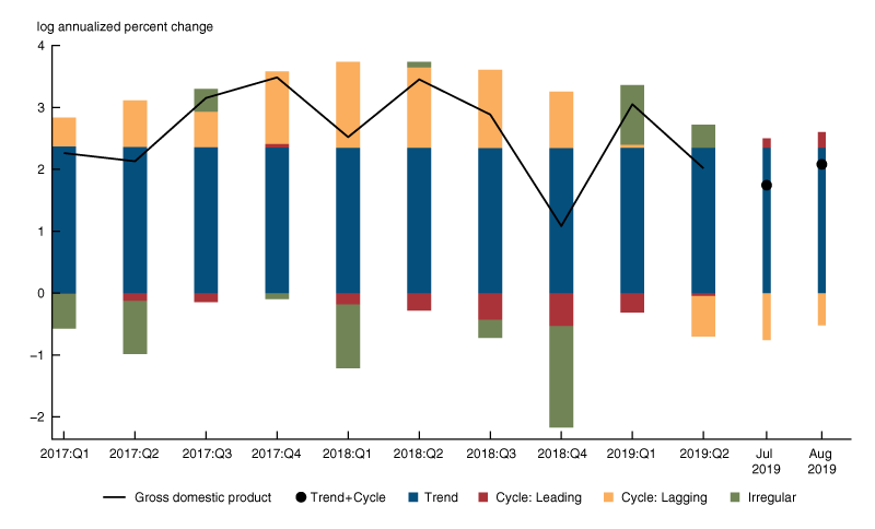
To conclude, we next summarize the model’s current results by decomposing in figure 6 quarterly real GDP growth since 2017 into estimated contributions from its trend, cycle, and irregular components. One can see from the figure that much of the above-trend growth in real GDP in 2017 and 2018 is attributed by the model to the cycle’s lagging subcomponent, with both the irregular component and leading subcomponent of the cycle often instead serving as drags on growth. The drag from the cycle’s leading subcomponent has since waned, and the contribution of the irregular component has pushed up growth so far in 2019.
6. Decomposition of real gross domestic product growth, 2017–19
Source: Authors’ calculations based on data from Haver Analytics.
The model estimates through August 2019 suggest that GDP growth is likely to be similar in the third quarter. Given the short-lived nature of the irregular component and its current downward trajectory, its positive effect on growth is not likely to persist for much longer, although we cannot verify this until we are able to observe its realized value when third quarter GDP is released on October 30, 2019. That said, August’s slightly smaller negative contribution from the cycle’s lagging subcomponent and the now slightly positive contribution from the cycle’s leading subcomponent suggest that real GDP growth in the third quarter is likely to be similar to what it was in the second quarter.
On November 4, 2019, updated estimates (through September 2019) of the Brave-Butters-Kelley Indexes (including BBK Monthly GDP Growth and the BBK Coincident and Leading Indexes) will be made available online, as will future monthly release dates.
1 Scott A. Brave, R. Andrew Butters, and David Kelley, 2019, “A new ‘big data’ index of U.S. economic activity,” Economic Perspectives, Federal Reserve Bank of Chicago, Vol. 43, No. 1. Crossref
2 A mixed-frequency collapsed dynamic factor model is a convenient statistical method of summarizing the correlation structure of a large panel of mixed-frequency (e.g., quarterly and monthly) time series into a small number of common “factors” explaining their evolution over time. For more information, see Brave, Butters, and Kelley (2019).
3 Brave, Butters, and Kelley (2019) compare the “big data” activity index to similar indexes such as the Chicago Fed National Activity Index and the Aruoba-Diebold-Scotti Business Conditions Index maintained by the Federal Reserve Bank of Philadelphia, and find that it aligns with historical U.S. recessions and expansions more accurately than both of these alternatives.
4 This feature is inherent to the way that the trend component of real GDP growth is modeled statistically as a “random walk,” where the best guess of what the trend will be in the next period is whatever it is currently.
5 We model this component as an independent and identically distributed (i.i.d.) normal random variable.
6 The cycle component is modeled as the sum of two subcomponents (leading and lagging), each with dynamics that are captured by stationary first-order autoregressions.
7 This threshold value is calculated by trading off the ratio of true positive and false positive classifications in exact proportion to the relative occurrence of expansions and recessions since 1960. This criterion equally penalizes false positive and false negative classifications of the business cycle. For further details, see Brave, Butters, and Kelley (2019).
8 For further explanation and additional examples of ROC analysis applied to business cycle indicators for the United States, see Travis J. Berge and Òscar Jordà, 2011, “Evaluating the classification of economic activity into recessions and expansions,” American Economic Journal: Macroeconomics, Vol. 3, No. 2, April, pp. 246–277. Crossref
9 This can be seen in panel B of figure 9 of Brave, Butters, and Kelley (2019).


